You’re walking down the street with your friend when a $50 bill floats down from the sky, flopping onto the sidewalk in front of you.

A few hours later, the two of you are staring each other down over a small bar table. The rules are final: the winner of a first-to-ten game of Heads or Tails will take the money. You’re up 8-7. As you prepare to flip the next coin, you hear a faint sound of screeching tires rapidly growing louder and louder. Suddenly, the room gets flooded with headlights and a car plows through the wall, sending bricks and beer everywhere. The game is abandoned without a winner. How do you share the money?¹

A slightly less dramatic version of this question was considered by two famous mathematicians, back in 1654. Through an exchange of letters, Pascal and Pierre de Fermat reasoned that in this situation, it would make sense to imagine that the game continued to the end (and there is a winner), and give each player a fraction of the money proportional to the number of final outcomes that they would have won. In our example, with a score of 8-7, you would win more of those outcomes (11 out of 16) than your friend, and so you should get $ \$50 \times\frac{11}{16} = \$ 34.38. $

These mathematicians basically reduced a philosophical problem (i.e., how to fairly redistribute the money) to one of counting, which turns out to be at the heart of all sorts of interesting problems in probability. Counting seems pretty straightforward in principle, but as with many things, the devil is in the details — depending on how and what you’re counting, you might be in for some mental trauma. In this article, I’ll go over the familiar idea of probability as the frequency of something happening, and introduce set theory as a language that allows for complex ideas to be modeled and manipulated in a very natural way. Nothing is assumed: we’ll go through everything you need right here.

Table of Contents

The meaning of probability

What does it mean to talk about the “probability” of something happening? Take a moment and think about the meaning of the word in these two sentences:

(a) the probability of your toast falling out of your plate and landing butter-side-up;
(b) the probability that the dog ate your homework.

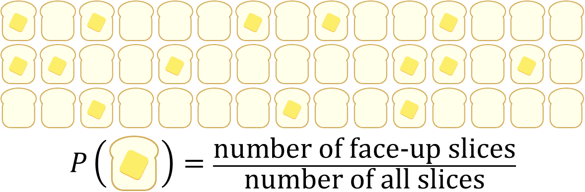
If you write the probability of (a) as $P(\textrm{falling toast lands butter-side-up}) = 0.3$, the usual interpretation might be something like, “if I dropped my toast a thousand times, the percentage of times that it would land butter-side-up would be around 30%”. In this situation, the meaning of probability is related to the frequency of something happening.

But what about (b)? It doesn’t really make sense to imagine a thousand rounds of the dog eating your homework. Here, $P(\textrm{dog ate homework}) = 0.999$ is a statement of your belief that the dog, with bits of lined paper stuck to his mouth, almost certainly had his way with your homework.

As you can see, the choice of interpretation depends on what you’re trying to model. In either case, by assigning a probability to something, we’re trying to describe a situation whose outcome is uncertain. We’ll start talking about the essential ingredients for such a description, and get you acquainted with a handful of terms that are common in probability.

Modeling uncertainty

To model an uncertain situation, or an experiment, we need to work out:

1. every possible thing that can happen, and
2. the probability of each thing happening.

The set of “every possible thing that can happen” is better known as the sample space, written as $\Omega$. In our “falling toast” situation, we could imagine that there are only two possible outcomes: (1) the toast lands butter-side-up (or “face-up”), denoted as $U$, or (2) it lands face-down, $D$. Then the sample space is the set of possibilities, $\Omega = \{U,D\}$.

Now let’s run through the probabilities for some “things that can happen”, which we define as events. We’re really talking about subsets of the sample space. There are only two possible events in our experiment, and so they both have non-zero probabilities. Since $P(\{U\}) = 0.3$, we know intuitively that $P(\{D\}) = P(\{\textrm{not }U\}) = 1-0.3 = 0.7$. There’s the (absolutely certain) event $\{U\textrm{ or } D\}$ that the toast lands either face-up or face-down, whose certainty is expressed as $P(\{U\textrm{ or } D\}) = 1$. We can also talk about impossible events, like the event that the toast lands simultaneously face-up and face-down, $\{U\textrm{ and } D\}$. This event is not in our sample space $\Omega$, so $P(\{U\textrm{ and } D\}) = 0$.

Let’s take a step back and ask ourselves: what is an event, really? And what does it mean exactly to say things like “and”, “or” and “not”? We’ve described events as being subsets of the sample space. This means that we can use the language of set theory to play around with events and express complex probabilistic situations with very little effort.

A segue into set theory

A set is an unordered, unique collection of items. Let’s say we have an experiment that involves drawing a card from a standard, shuffled 52-card deck, with four suits (Clubs, Spades, Hearts, Diamonds) and thirteen ranks. In this case, the sample space $\Omega$ (the set of all cards in the deck) is one such set. Another set could be the collection of Heart and Diamond face cards,

$$ S = \left\{ K\heartsuit, Q\heartsuit, J\heartsuit, K\diamondsuit, Q\diamondsuit, J\diamondsuit \right\}. $$

We would say that this is a 6-element subset of the 52-element sample space $\Omega$, because every element in $S$ can be found in $\Omega$. The number of elements in $S$ is written as $|S| = 6$. A set that has no elements is equivalent to the empty set, denoted by the $ \emptyset $ symbol.

Take note of the definition: a set is an unordered and unique collection of items. That means the order in which you list the items of a set doesn’t matter, and there can be no duplicates of an element.

Set operations

Now we can start talking about manipulating sets. Although there are many ways to model an uncertain situation, some are more convenient than others. Generally, we like to play with sets that can be expressed concisely, and more importantly, allow us to avoid hard probability computations. Set operations are the tools that allow us to sculpt exactly the kinds of sets we want.

The complement (“not”) operation is as simple as it is useful. With respect to the sample space $\Omega$, the complement of $S$ (written as $S^\complement$), is the set of all elements in $\Omega$ that are not in $S$. Imagine if you wanted to find the probability of “anything other than a black King”. You would probably much prefer to write this as $P(\{\textrm{black king}\}^\complement)$ or $P(\textrm{not black king})$, rather than listing every non-black-King card in a set. The complement of $\Omega$ is the empty set, $\emptyset$. Likewise, $\emptyset^\complement = \Omega$.

The union of two sets $A$ and $B$ is the set of all elements in $\Omega$ that belong to either $A$ or $B$, inclusive. Using a little notation, we would write

$$ A \cup B = \{x | x \textrm{ is in } A \textbf{ or } x \textrm{ is in } B\}, $$

where the vertical line reads “such that”.

The intersection of $A$ and $B$ is the set of all elements in $\Omega$ that are in both $A$ and $B$.

$$ A \cap B = \{x | x \textrm{ is in } A \textbf{ and } x \textrm{ is in } B\} $$

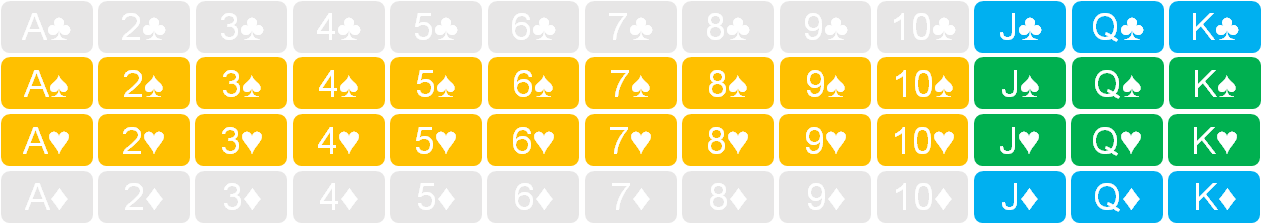
We can visualize the union and intersection sets with a couple of examples: $A$, the set of face cards, and $B$, the set of all Hearts and Clubs. The figure below shows cards that only belong to $A$ in yellow, and those exclusive to $B$ in blue. The cards common to both sets, shown in green, are the elements of the intersection $A \cap B$. The union of the two sets, $A \cup B$ is the set of all yellow, green, and blue cards.

De Morgan’s laws

In the last example we can express the cards that do not belong to either set (grey cards in Fig. 2) as $(A \cup B)^\complement$. Depending on the problem, you might find it easier to work out the probability of an intersection (or a union). We can alternate between intersections and unions using De Morgan’s laws:

$$ (A_{1} \cup A_{2} \cup … \cup A_{n})^\complement = A_{1}^\complement \cap A_{2}^\complement \cap … \cap A_{n}^\complement $$ $$ (A_{1} \cap A_{2} \cap … \cap A_{n})^\complement = A_{1}^\complement \cup A_{2}^\complement \cup … \cup A_{n}^\complement $$

What are these saying in English? $(A \cup B)^\complement$ is translated as “everything other than $A$ or $B$”, whereas $A^\complement \cap B^\complement$ can be read as “not A and not B”. Of course, these two are logically equivalent.

So, we can use De Morgan’s laws to switch between different representations of the same set. Don’t worry if this seems a bit abstract right now — we’ll see later on how this can be useful.

Partitions and disjoint sets

We’ll round out our whirlwind tour of set theory with a brief discussion about partitions, which are a collection of subsets of some set that (a) have nothing in common with each other, and (b) completely exhaust (or account for) that set. You will often find yourself carving the sample space into partitions to work out the probability of some event. They also help in making sure your probability math checks out.

The sample space of our card-drawing experiment can be split into a few different partitions. Here are a few examples:

$$ \begin{align} \Omega &= \{\textrm{red suits}\} \cup \{\textrm{black suits}\} \\\
&= \{\textrm{clubs}\} \cup \{\textrm{spades}\} \cup \{\textrm{hearts}\} \cup \{\textrm{diamonds}\} \\\
&= \{\textrm{even rank}\} \cup \{\textrm{odd rank}\} \\\
&= \{\textrm{rank } \leq 4\} \cup \{\textrm{rank } > 4\} \end{align} $$

We can see that in each partition, the intersection of any two sets is the empty set, and all elements of $\Omega$ are accounted for by their union. Note that when $A \cap B = \emptyset$, we say that $A$ and $B$ are disjoint, or mutually exclusive.

There’s nothing stopping us from making useless partitions — any collection of sets that satisfies the two listed restrictions can be a partition. That said, you’ll usually want to split the sample space in a way that makes solving your problem easier.

With some set theory under our belt, we’re ready to return to the world of probability. Counting the number of things in sets is at the heart of probability, and naturally leads to its oldest and most familiar definition.

Naive definition of probability

The probability of an event, if each experiment outcome is equally likely, can be worked out by counting the number of ways it could happen, and then dividing by the total number of outcomes.

$$ P(E) = \frac{\textrm{number of favorable outcomes}}{\textrm{total number of outcomes}} $$

When our assumption that every outcome has equal probability is justified (as when drawing a card from a well-shuffled, standard deck of cards), we can compute probabilities very easily. The probability of drawing a Diamond becomes $P(\textrm{diamond}) = \frac{\textrm{number of diamonds}}{\textrm{number of cards in deck}} = \frac{13}{52}$. In general, when there are $n$ elements in the sample space $\Omega$, and event $E$ is a k-element subset of $\Omega$,

$$P(E) = \frac{|E|}{|\Omega|} = \frac{k}{n},$$

where $|S|$ is the number of elements in set $S$.

About that assumption

It’s easy to see how the naive definition breaks down when our “all outcomes have equal likelihood” assumption is not valid. Going back to our falling toast experiment, we have two outcomes: butter-side up, with $P(U) = 0.3$, and butter-side-down, with $P(D) = 0.7$. If we wanted to calculate $P(U)$ using the naive definition, we’d get 1/2, which we know to be wrong.

A more fundamental limitation is that this definition relies on events that are finite and countable. It wouldn’t make sense to count the number of elements in an “all even integers” event, for example.

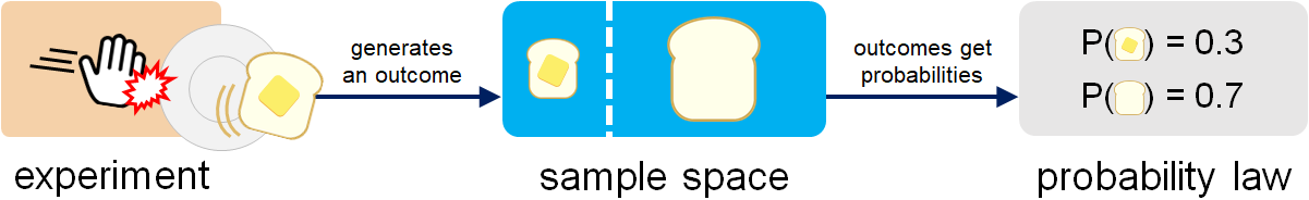
Building a probability model

Here’s a (mostly familiar) list of what we need to build a probability model:

1. An experiment, a process that results in some kind of outcome,
2. The sample space, containing all possible outcomes of the experiment,
3. A probability law that assigns probability to each possible outcome.

Our “falling toast” example has all of these: (1) an experiment (e.g., you knock the plate and the toast falls off the table), (2) a sample space $\Omega = \{U,D\}$, and the probability of each outcome.

Take a look at the sketch of the sample space above: it looks like the two possible outcomes are taking up different amounts of the sample space, in proportion to their probability. In fact, it’s useful to think about the outcomes as taking up some amount of the total available probability. We’ll explore this idea very soon.

A quick note on experiments

Up until now our experiments have involved single, one-shot happenings: drawing a card, and dropping a slice of toast. But there’s nothing stopping us from using more complicated experiments. For sequential experiments, like flipping a coin five times, each outcome is the result of multiple sub-outcomes chained together. Here, each element of $\Omega$ will look like $(c_{1},c_{2},c_{3},c_{4},c_{5})$, or $c_{1}c_{2}c_{3}c_{4}c_{5}$, where $c_{n}$ stands for the sub-outcome of the $n$th coin flip. We could then talk about the probability of an outcome like “getting four Heads in a row”, $P(HHHHT \textrm{ or } THHHH)$.

The sample spaces for sequential experiments tend to be quite a lot larger than their one-shot counterparts. To give you an idea, a single coin flip has only two possible outcomes, Heads and Tails, while the sample space for the “five coin flips” experiment has $|\Omega| = 2^5 = 32$ outcomes.

Choosing your sample space

When deciding how to model your sample space, you need to ensure three things:

1. the sample space is collectively exhaustive (accounts for every possible outcome),
2. the elements are mutually exclusive (each element in the sample space is unique),
3. the sample space is appropriately “granular”.

That last point could do with some explanation. Let’s dial it up to 11 for a second¹.

In our falling toast experiment, we chose a sample space of $\Omega = \{U,D\}$ because we were interested in whether the slice lands face-up or face-down. But imagine a situation in which a mischievous spirit has possessed our toaster. Now, the toaster launches buttered bread, out of the toaster and onto the floor. Not only that, the spirit has taken control of the toaster’s heat setting, randomly using one of three heat levels for each slice of bread.

Assuming you had a (slightly bizarre) interest in modeling this new experiment, you could choose a sample space $\Omega^{*}$ that has elements like $(r,h)$, where $r \in \{U,D\}$ is the face-up-or-down result, and $h \in \{H_{1}, H_{2}, H_{3}\}$ represents the heat level.

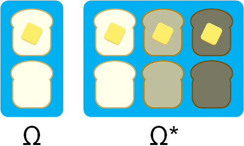
Since $\Omega^{*}$ has just enough complexity to be used in our heat investigation, this sample space has the right level of granularity. On the other hand, the original $\Omega$ is not granular enough. You should choose a sample space that captures what you’re interested in — and nothing more.

Assigning probability

A probability law allocates probability to experiment outcomes. What are the rules for how this can be done? Up until now we’ve tiptoed around these rules, abiding by them but never really mentioning them. It’s time to change that. This section will go over the three fundamental axioms that underlie all of probability, and what this means for our calculations.

Probability axioms

Imagine that the sample space is a cake whose weight is measured as one unit of probability. Each event $E$ is a slice of cake that has weight $P(E)$. This leads us to our first axiom, which says that this weight cannot be negative:

$$\textbf{A1. } P(E) \geq 0 \textrm{ for event } E.$$

The second axiom says that for two disjoint events (or two separate pieces of cake), their total weight is the sum of their individual weights:

$$\textbf{A2. } P(E_{1} \cup E_{2}) = P(E_{1}) + P(E_{2}).$$

The third and final axiom says that the total weight of the sample space (cake) is one probability unit:

$$\textbf{A3. } P(\Omega) = 1.$$

Properties of probability

We can use the three axioms to derive all sorts of intuitive findings about probability, which we’ll explore using some examples. It’s worth spending some time with these to make sure you understand them, as they will crop up over and over again as you work with probability models.

One of the most useful (and familiar) findings states that if the sample space consists of a finite number of unique elements $e_{i}$, we can work out the probability of any event $E = \{e_{1} \cup e_{2} \cup … \cup e_{n}\}$ by summing the probabilities of its elements:

$$P(E) = P(e_{1}) + P(e_{2}) + … + P(e_{n}) = \sum_{i=1}^{n} P(e_{i})$$

As a quick example, you can work out the probability of drawing a Spade face card by applying Axiom 2 and summing the individual probabilities,

$$P(J\spadesuit \cup Q\spadesuit \cup K\spadesuit) = P(J\spadesuit) + P(Q\spadesuit) + P(K\spadesuit) = \frac{3}{52}.$$

Model A: flipping a fair coin

Here we’re dealing with two equally likely outcomes, Heads or Tails, and so the sample space consists of two elements, $\Omega = \{H,T\}$. The set of all possible events is

$$\{H\}, \{T\}, \{H \cup T\}, \emptyset$$

Let’s work out the probability of each event using the axioms.

• By definition, $P(H) = P(T) = 0.5$.
• We know that a coin cannot show both Heads and Tails, which means $H$ and $T$ are disjoint and $P(H \cup T) = P(H) + P(T)$.
• Since $H$ and $T$ are the only outcomes, the sets $\{H\}$ and $\{T\}$ are a partition for $\Omega$. That means $P(H \cup T) = P(\Omega) = 1$.

What about $P(\emptyset)$? Since $\emptyset$ and $\Omega$ are disjoint, we can work out

$$P(\emptyset \cup \Omega) = P(\emptyset) + P(\Omega) = P(\emptyset) + 1.$$

Since probability can’t be negative (or larger than 1), this tells us that $P(\emptyset) = 0$.

The probability law (i.e., the assignment of probability for every event) thus falls out from a straightforward application of the axioms:

$$P(H) = 0.5, P(T) = 0.5, P(\Omega) = P(H \cup T) = 1, P(\emptyset) = 0$$

Model B: flipping an unfair toast, twice

We return to our falling toast experiment, but with a wrinkle: we’re interested in the outcome of two consecutive toast ‘flips’. That means we’re now dealing with a sequential model, with sample space

$$\Omega = \{DD, DU, UD, UU\}.$$

How do we compute $P\{DU\}$? The outcome $DU$ means that we got face-down on the first flip and face-up on the second. We know that $P(U) = 0.3$ and $P(D) = 0.7$. Since the outcome of the first flip has nothing to do with the outcome of the second (and vice versa), we can compute the probability like this:

$$P(DU) = P(D) \times P(U) = 0.7 \times 0.3 = 0.21.$$

Similarly, we can work out all the other probabilities, making sure that their sum accounts for the entire weight of the sample space,

$$ \begin{align} \sum_{i=1}^{4} P(e_{i}) &= P(DD) + P(DU) + P(UD) + P(UU) \\\
&= 0.09 + 0.21 + 0.21 + 0.49 = 1 = P(\Omega). \end{align} $$

How would we compute the probability of ending up with at least one face-up slice of toast? We’re interested in the probability that we get one face-up slice or two face-up slices. That’s just a matter of summing the probability of all outcomes that lead to this particular result:

$$ \begin{align} P(\textrm{at least one face-up}) &= P(DU \cup UD \cup UU) \\\
&= P(DU) + P(UD) + P(UU) \\\
&= 0.21 + 0.21 + 0.09 = 0.51. \end{align}\\\\\\\\$$

Summary

And there you have it: an introduction to set theory as the language of probability. Playing around with sets might seem a little dry, but remember: you’re dealing with a language, and fluency in this language will allow you to better express and reason about all sorts of interesting probabilistic situations.

What kinds of situations, you ask? That’s for you to decide!